There are many possible depreciation methods, but straight-line and double-declining balance are the most popular. In addition, the units-of-output method is uniquely suited to certain types of assets. The following discussion covers each of these methods. Intermediate accounting courses typically introduce additional techniques that are sometimes appropriate.
The Straight-Line Method
Under the straight-line approach the annual depreciation is calculated by dividing the depreciable base by the service life. To illustrate assume that an asset has a $100,000 cost, $10,000 salvage value, and a four-year life. The following schedule reveals the annual depreciation expense, the resulting accumulated depreciation at the end of each year, and the related calculations.
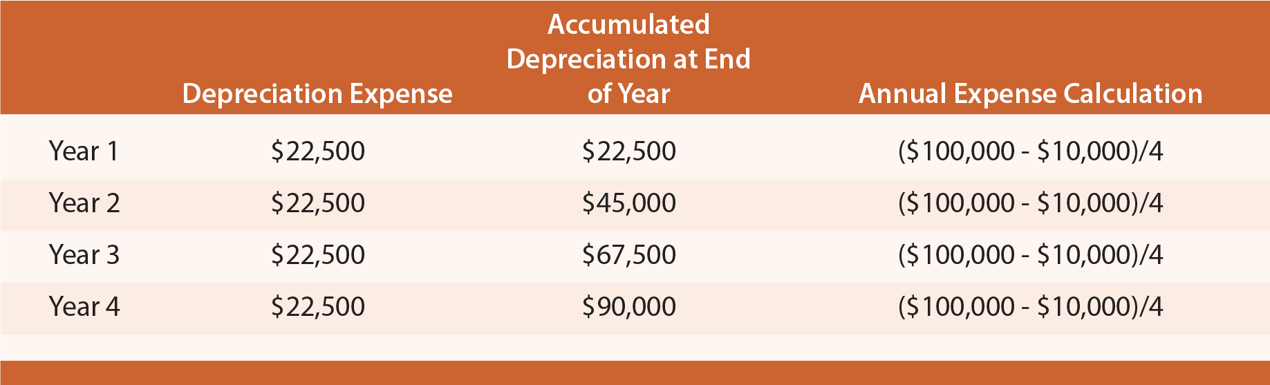
For each of the above years, the journal entry to record depreciation is as follows:
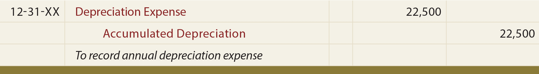
The applicable depreciation expense would be included in each year’s income statement (except in a manufacturing environment where some depreciation may be assigned to the manufactured inventory, as explained in managerial accounting courses). The appropriate balance sheet presentation would appear as follows (end of year 3 in this case):

Fractional Period Depreciation (SL)
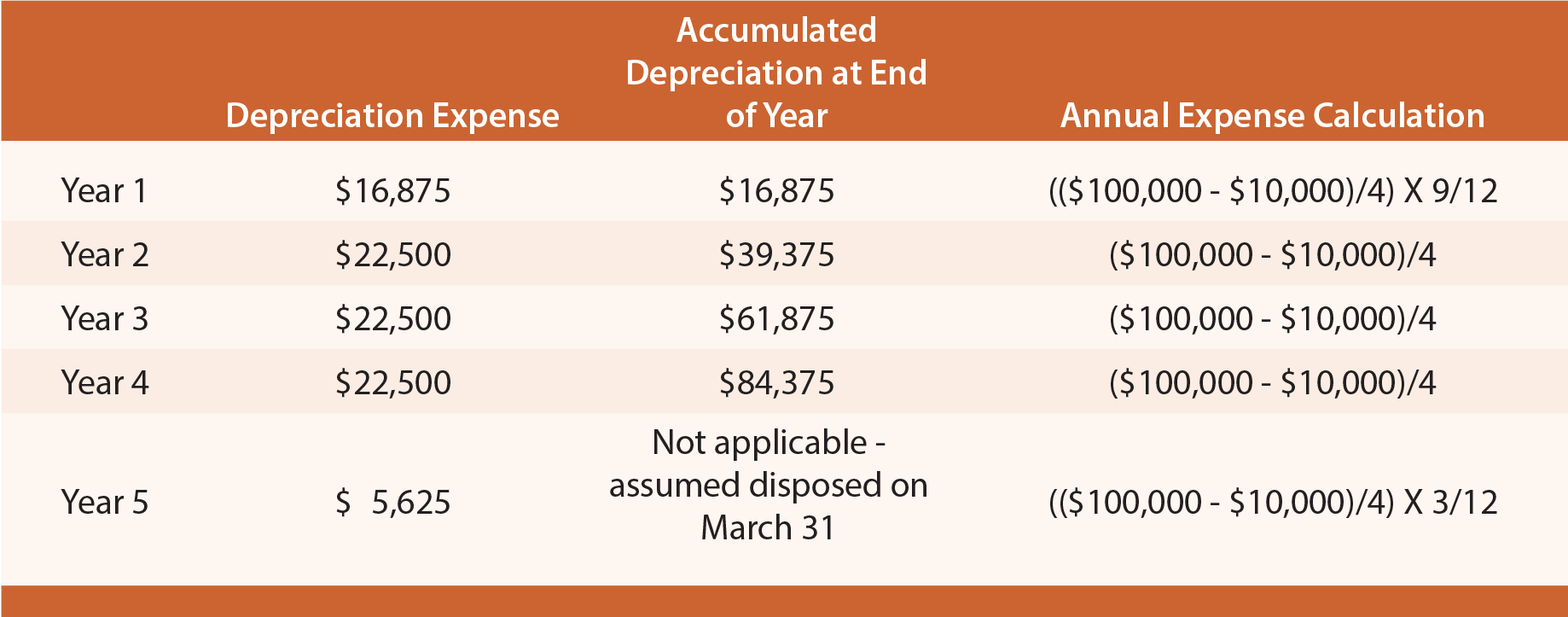
Assets may be acquired at other than the beginning of an accounting period. Some companies simply assume that these assets are acquired at the beginning or end of the period. Other companies will calculate depreciation for partial periods. With the straight-line method the partial-period depreciation is simply a fraction of the annual amount. For example, an asset acquired on the first day of April would be used for only nine months during the first calendar year. Therefore, Year 1 depreciation would be 9/12 of the annual amount. Following is the depreciation table for the asset, this time assuming an April 1st acquisition date:
Spreadsheet Software (SL)
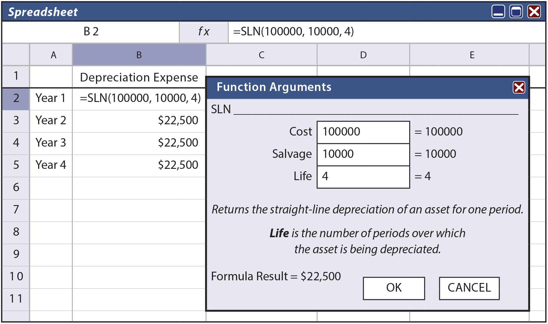
Computer-based spreadsheets usually include built-in depreciation functions. Below is a screen shot showing the straight-line method. Data are entered in the query form, and the routine returns the formula and annual depreciation value to the selected cell of the worksheet.
The Units-of-Output Method
The units-of-output method involves calculations that are quite similar to the straight-line method, but it allocates the depreciable base over the units of output rather than years of use. It is logical to use this approach in those situations where the life is best measured by identifiable units of machine “consumption.” For example, perhaps the engine of a corporate jet has an estimated life of 50,000 hours. Or, a printing machine may produce an expected 4,000,000 copies. In cases like these, the accountant may opt for the units-of-output method.
To illustrate, assume Dat Nguyen Painting Corporation purchased an air filtration system that has a life of 8,000 hours. The filter cost $100,000 and has a $10,000 salvage value. Nguyen anticipates that the filter will be used 1,000 hours during the first year, 3,000 hours during the second, 2,000 during the third, and 2,000 during the fourth. Accordingly, the anticipated depreciation schedule would appear as follows (if actual usage varies, the schedule would be adjusted for the changing estimates using principles that are discussed later in this chapter):
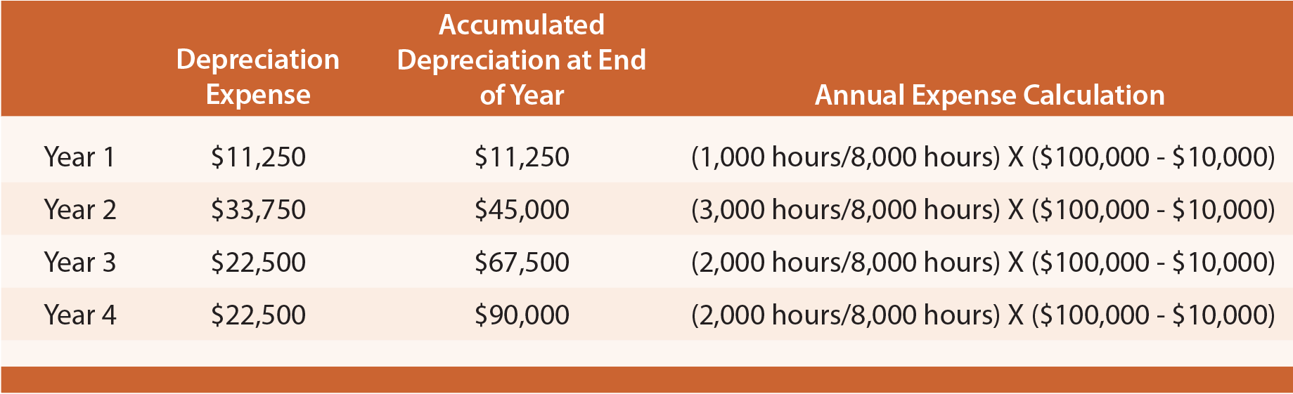
The form of journal entry and balance sheet account presentation are just like the straight-line illustration, but with the revised amounts from this table.
The Double-Declining Balance Method
As one of several accelerated depreciation methods, double-declining balance (DDB) results in relatively large amounts of depreciation in early years of asset life and smaller amounts in later years. This method can be justified if the quality of service produced by an asset declines over time, or if repair and maintenance costs will rise over time to offset the declining depreciation amount.
With this method, 200% of the straight-line rate is multiplied times the remaining book value of an asset (as of the beginning of a particular year) to determine depreciation for a particular year. As time passes, book value and annual depreciation decrease. To illustrate, again utilize the example of the $100,000 asset, with a four-year life, and $10,000 salvage value. Depreciation for each of the four years would appear as follows:
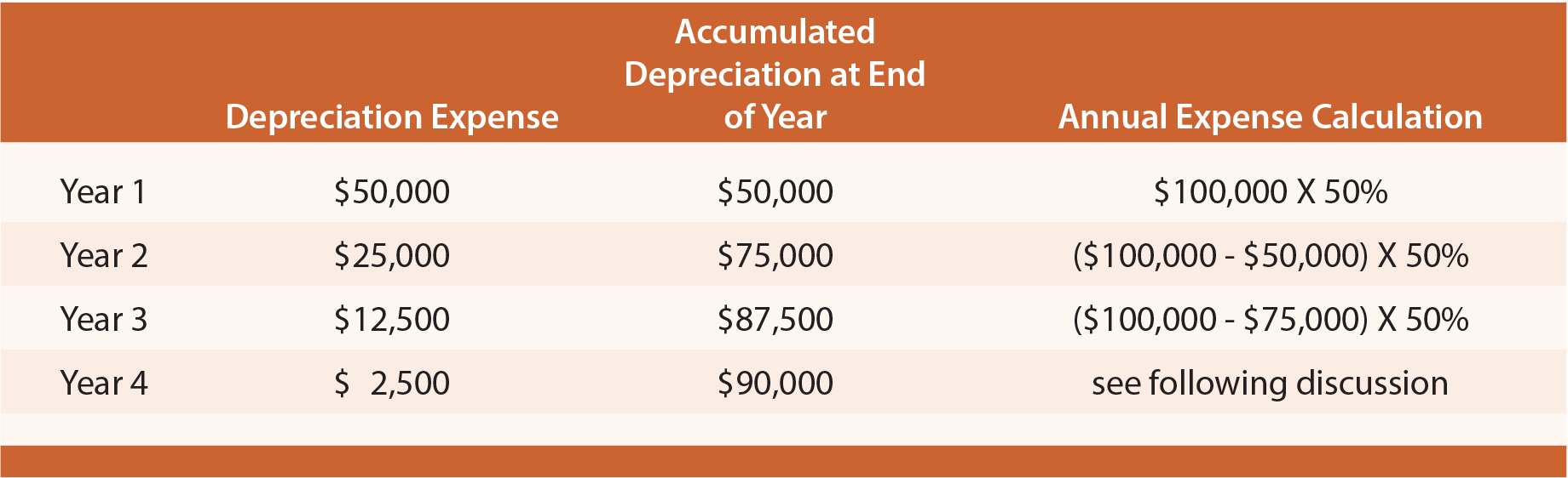
The amounts in the above table deserve additional commentary. Year 1 expense equals the cost times twice the straight-line rate (four-year life = 25% straight-line rate; 25% X 2 = 50% rate). Year 2 is the 50% rate applied to the beginning of year book value. Year 3 is calculated in a similar fashion.
Note that salvage value was ignored in the preliminary years’ calculations. For Year 4, however, the calculated amount (($100,000 – $87,500) X 50% = $6,250) would cause the lifetime depreciation to exceed the $90,000 depreciable base. Thus, in Year 4, only $2,500 is taken as expense. This gives rise to an important general rule for DDB: salvage value is initially ignored, but once accumulated depreciation reaches the amount of the depreciable base, then depreciation ceases. In the example, only $2,500 was needed in Year 4 to bring the aggregate depreciation up to the $90,000 level.
An asset may have no salvage value. The mathematics of DDB will never fully depreciate such assets (since one is only depreciating a percentage of the remaining balance, the remaining balance would never go to zero). In these cases, accountants typically change to the straight-line method near the end of an asset’s useful life to “finish off” the depreciation of the asset’s cost.
Spreadsheet Software (DDB)
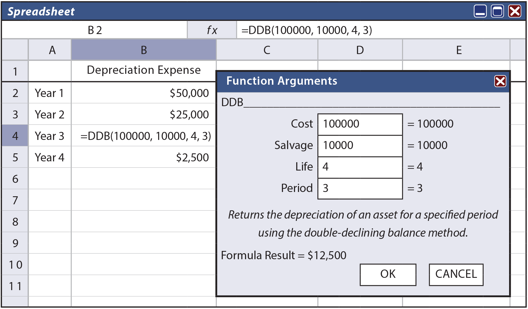
DDB is also calculable from spreadsheet depreciation functions. Below is a routine that returns the $12,500 annual depreciation value for Year 3.
Fractional Period Depreciation (DDB)
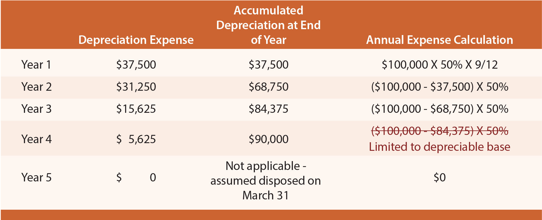
Under DDB, fractional years involve a very simple adaptation. The first partial year will be a fraction of the annual amount, and all subsequent years will be the normal calculation (twice the straight-line rate times the beginning of year book value). If the example asset was purchased on April 1st of Year 1, the following calculations result:
Alternatives to DDB
150% and 125% declining balance methods are quite similar to DDB, but the rate is 150% or 125% of the straight-line rate (instead of 200% as with DDB).
Changes in Estimates
Obviously, the initial assumption about useful life and residual value is only an estimate. Time and new information may suggest that the initial assumptions need to be revised, especially if the initial estimates prove to be materially off course. It is well accepted that changes in estimates do not require restating the prior period financial statements; after all, an estimate is just that, and the financial statements of prior periods were presumably based on the best information available at the time. Therefore, such revisions are made prospectively (over the future) so that the remaining depreciable base is spread over the remaining life.
To illustrate, reconsider the straight-line method. Assume that two years have passed for the $100,000 asset that was initially believed to have a four-year life and $10,000 salvage value. As of the beginning of Year 3, new information suggests that the asset will have a total life of seven years (three more than originally thought), and a $5,000 salvage value. As a result, the revised remaining depreciable base (as of the beginning of Year 3) will be spread over the remaining five years, as follows:
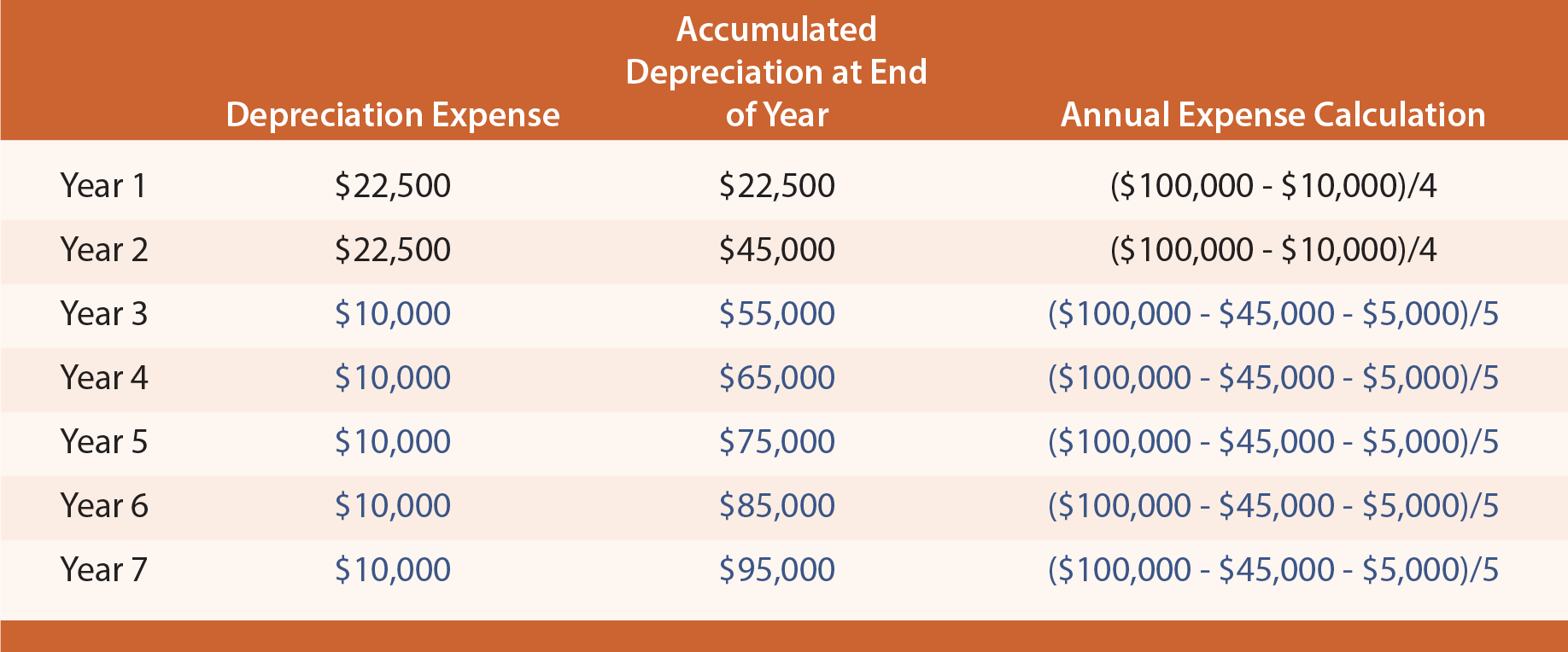
Depreciation for Years 3 through 7 is based on spreading the “revised” depreciable base over the last five years of remaining life. The “revised” depreciable base is $50,000. It is computed as the original cost, minus the previous depreciation ($45,000), and minus the revised salvage value ($5,000).
Asset Revaluation
International accounting and reporting standards include provisions that permit companies to revalue items of PP&E to fair value. When applied, all assets in the same class must be revalued annually. Such balance sheet adjustments are offset with a corresponding change in the entity’s capital accounts. These revaluations pose additional complications because they result in continuous alterations of the amount of depreciation.
| Did you learn? |
|---|
| Apply the straight-line method of depreciation, including situations involving partial periods. |
| Apply the units-of-output method of depreciation. |
| Apply the declining-balance method of depreciation, including situations involving partial periods. |
| Be aware of declining-balance alternatives, such as 200%, 150%, and 125% rates. |
| Know that electronic spreadsheets usually have built-in functions supporting depreciation calculations. |
| How are changes in estimates (e.g., useful life) dealt with in the basic depreciation computations? |
| Recognize that global approaches vary, and assets are sometimes revalued in global reporting. |