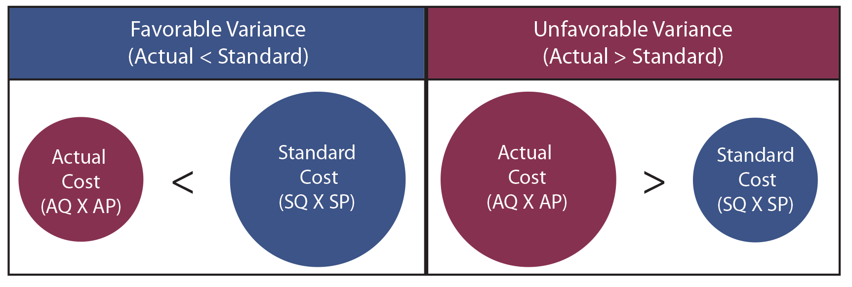
Standard costs provide information that is useful in performance evaluation. Standard costs are compared to actual costs, and mathematical deviations between the two are termed variances. Favorable variances result when actual costs are less than standard costs, and vice versa. The following illustration is intended to demonstrate the very basic relationship between actual cost and standard cost. AQ means the “actual quantity” of input used to produce the output. AP means the “actual price” of the input used to produce the output. SQ and SP refer to the “standard” quantity and price that was anticipated. Variance analysis can be conducted for material, labor, and overhead.
Direct Material Variances
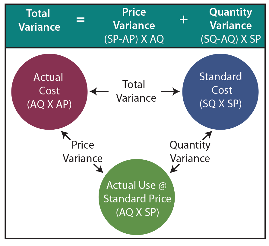 Management is responsible for evaluation of variances. This task is an important part of effective control of an organization. When total actual costs differ from total standard costs, management must perform a more penetrating analysis to determine the root cause of the variances. The total variance for direct materials is found by comparing actual direct material cost to standard direct material cost. However, the overall materials variance could result from any combination of having procured goods at prices equal to, above, or below standard cost, and using more or less direct materials than anticipated. Proper variance analysis requires that the Total Direct Materials Variance be separated into the:
- Materials Price Variance: A variance that reveals the difference between the standard price for materials purchased and the amount actually paid for those materials [(standard price – actual price) X actual quantity].
- Materials Quantity Variance: A variance that compares the standard quantity of materials that should have been used to the actual quantity of materials used. The quantity variation is measured at the standard price per unit [(standard quantity – actual quantity) X standard price].
Note that there are several ways to perform the intrinsic variance calculations. One can compute the values for the red, blue, and green balls and note the differences. Or, one can perform the algebraic calculations for the price and quantity variances. Note that unfavorable variances (negative) offset favorable (positive) variances. A total variance could be zero, resulting from favorable pricing that was wiped out by waste. A good manager would want to take corrective action, but would be unaware of the problem based on an overall budget versus actual comparison.
Case Study
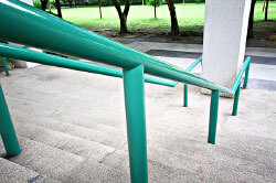 Blue Rail produces handrails, banisters, and similar welded products. The primary raw material is 40-foot long pieces of steel pipe. This pipe is custom cut and welded into rails like that shown in the accompanying picture. In addition, the final stages of production require grinding and sanding operations, along with a final coating of paint (welding rods, grinding disks, and paint are relatively inexpensive and are classified as indirect material within factory overhead).
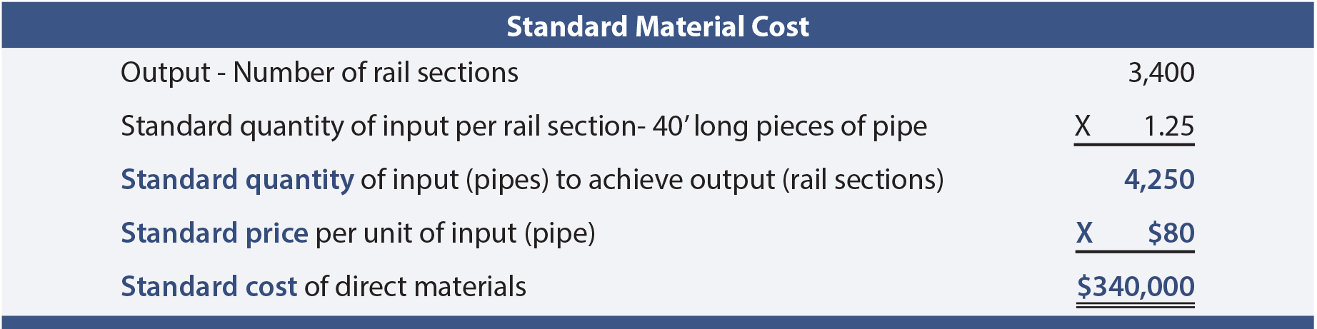
Blue Rail measures its output in “sections.” Each section consists of one post and four rails. The sections are 10’ in length and the posts average 4’ each. Some overage and waste is expected due to the need for an extra post at the end of a set of sections, faulty welds, and bad pipe cuts. The company has adopted an achievable standard of 1.25 pieces of raw pipe (50’) per section of rail. During August, Blue Rail produced 3,400 sections of railing. It was anticipated that pipe would cost $80 per 40’ piece. Standard material cost for this level of output is computed as follows:
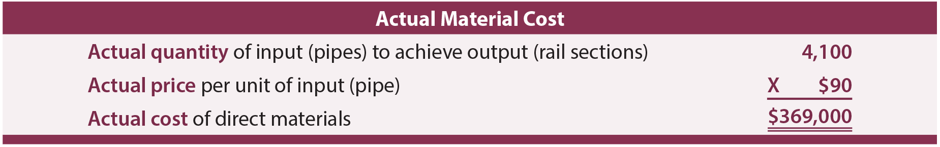
The production manager was disappointed to receive the monthly performance report revealing actual material cost of $369,000. A closer examination of the actual cost of materials follows.
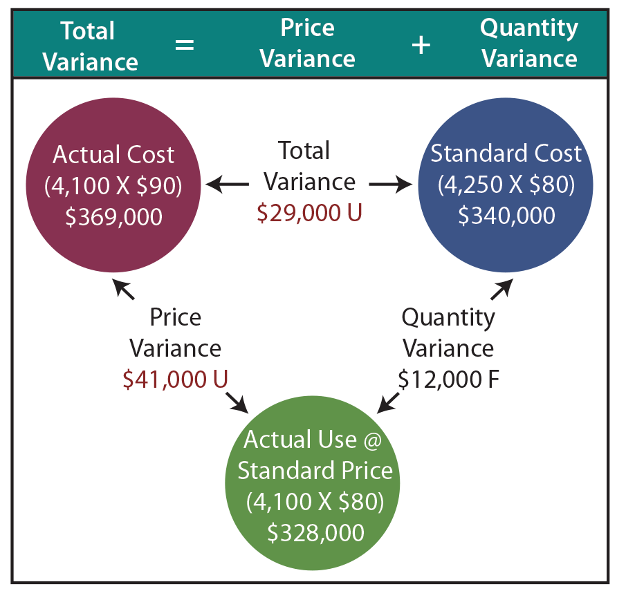
The total direct material variance was unfavorable $29,000 ($340,000 vs. $369,000). However, this unfavorable outcome was driven by higher prices for raw material, not waste, as follows:
MATERIALS PRICE VARIANCE
(SP – AP) X AQ = ($80 – $90) X 4,100
= <$41,000>
Materials usage was favorable since less material was used (4,100 pieces of pipe) than was standard (4,250 pieces of pipe). This resulted in a favorable materials quantity variance:
MATERIALS QUANTITY VARIANCE
(SQ – AQ) X SP = (4,250 – 4,100) X $80
=$12,000
Journal Entries
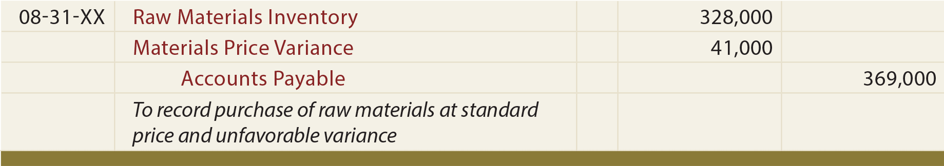
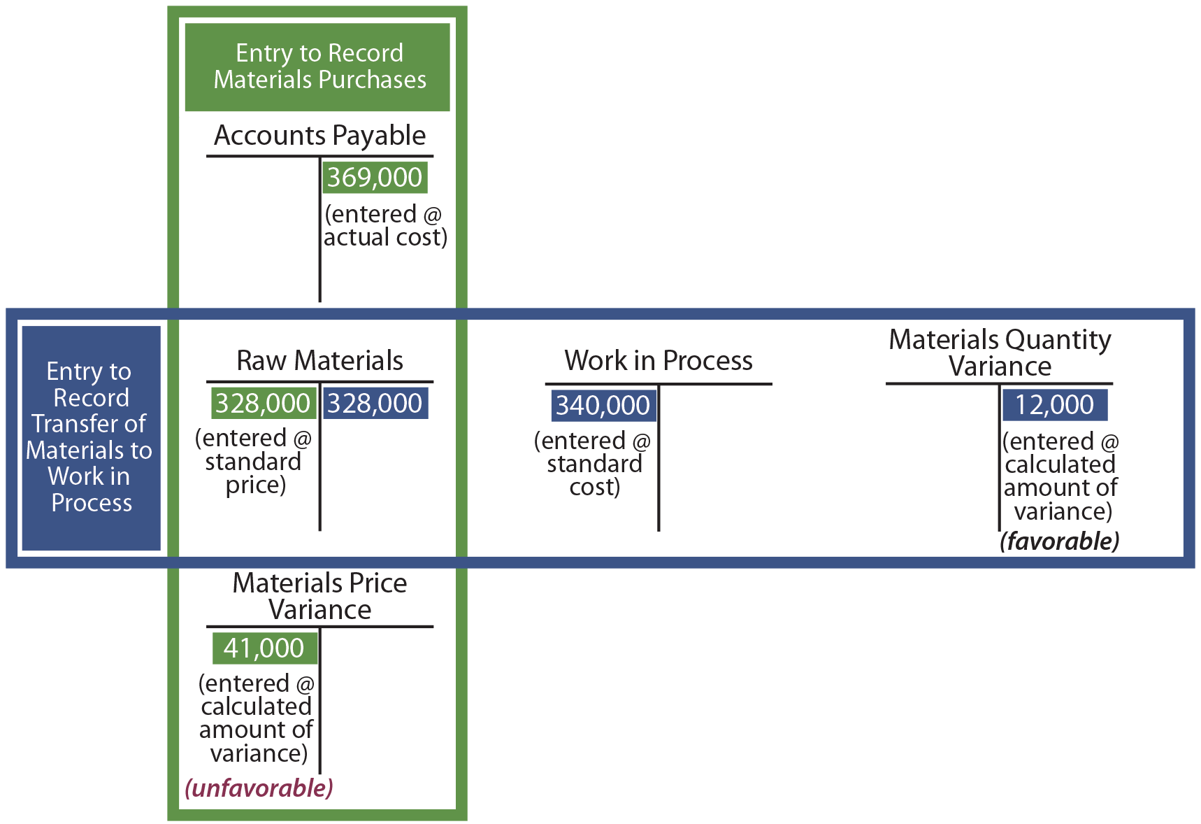
A company may desire to adapt its general ledger accounting system to capture and report variances. Do not lose sight of the very simple fact that the amount of money to account for is still the money that was actually spent ($369,000). To the extent the price paid for materials differs from standard, the variance is debited (unfavorable) or credited (favorable) to a Materials Price Variance account. This results in the Raw Materials Inventory account carrying only the standard price of materials, no matter the price paid:
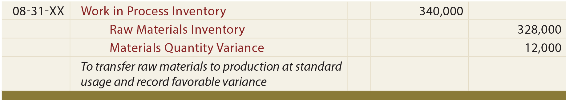
Work in Process is debited for the standard cost of the standard quantity that should be used for the productive output achieved, no matter how much is used. Any difference between standard and actual raw material usage is debited (unfavorable) or credited (favorable) to the Materials Quantity Variance account:
The price and quantity variances are generally reported by decreasing income (if unfavorable debits) or increasing income (if favorable credits), although other outcomes are possible. Examine the following diagram and notice the $369,000 of cost is ultimately attributed to work in process ($340,000 debit), materials price variance ($41,000 debit), and materials quantity variance ($12,000 credit). This illustration presumes that all raw materials purchased are put into production. If this were not the case, then the price variances would be based on the amount purchased while the quantity variances would be based on output.
Direct Labor Variances
 The logic for direct labor variances is very similar to that of direct material. The total variance for direct labor is found by comparing actual direct labor cost to standard direct labor cost. If actual cost exceeds standard cost, the resulting variances are unfavorable and vice versa. The overall labor variance could result from any combination of having paid laborers at rates equal to, above, or below standard rates, and using more or less direct labor hours than anticipated.
In this illustration, AH is the actual hours worked, AR is the actual labor rate per hour, SR is the standard labor rate per hour, and SH is the standard hours for the output achieved.
The Total Direct Labor Variance consists of:
- Labor Rate Variance: A variance that reveals the difference between the standard rate and actual rate for the actual labor hours worked [(standard rate – actual rate) X actual hours].
- Labor Efficiency Variance: A variance that compares the standard hours of direct labor that should have been used to the actual hours worked. The efficiency variance is measured at the standard rate per hour [(standard hours – actual hours) X standard rate].
As with material variances, there are several ways to perform the intrinsic labor variance calculations. One can compute the values for the red, blue, and green balls. Or, one can perform the noted algebraic calculations for the rate and efficiency variances.
Case Study
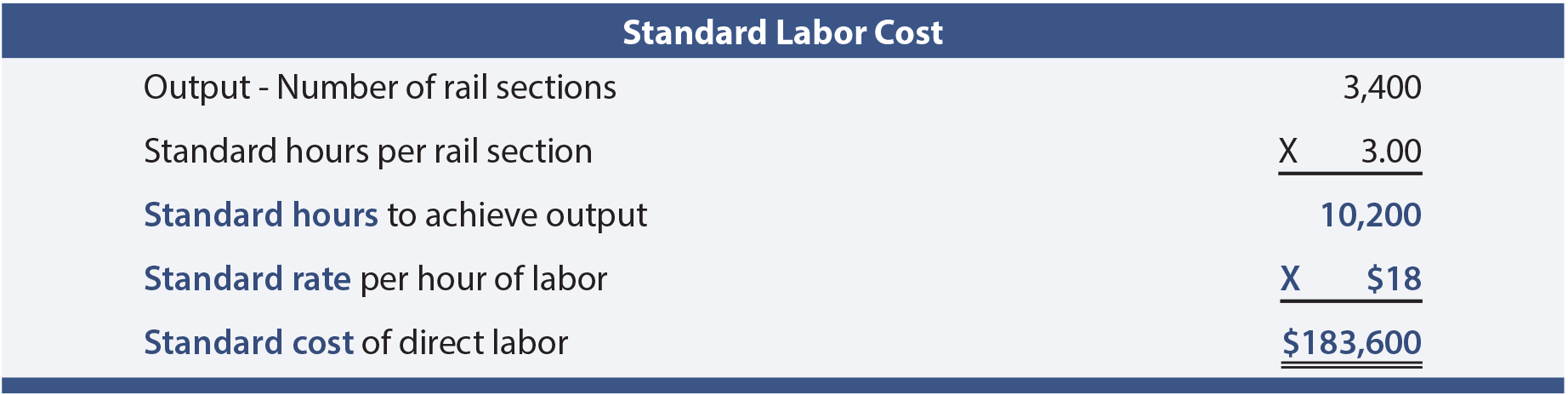
Recall that Blue Rail Manufacturing had to custom cut, weld, sand, and paint each section of railing. The company has adopted a standard of 3 labor hours for each section of rail. Skilled labor is anticipated to cost $18 per hour. During August, remember that Blue Rail produced 3,400 sections of railing. Therefore, the standard labor cost for August is calculated as:
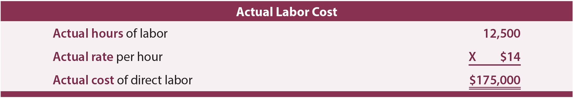
The monthly performance report revealed actual labor cost of $175,000. A closer examination of the actual cost of labor revealed the following:
The total direct labor variance was favorable $8,600 ($183,600 vs. $175,000). However, detailed variance analysis is necessary to fully assess the nature of the labor variance. As will be shown, Blue Rail experienced a very favorable labor rate variance, but this was offset by significant unfavorable labor efficiency.
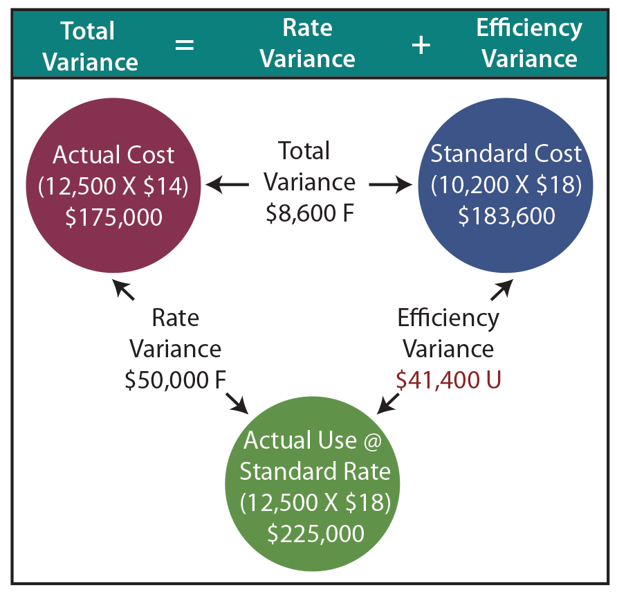
LABOR RATE VARIANCE
(SR – AR) X AH = ($18 – $14) X 12,500
= $50,000
The hourly wage rate was lower because of a shortage of skilled welders. Less-experienced welders were paid less per hour, but they also worked slower. This inefficiency shows up in the unfavorable labor efficiency variance:
LABOR EFFICIENCY VARIANCE
(SH – AH) X SR = (10,200 – 12,500) X $18
=<$41,400>
Journal Entry
If Blue Rail desires to capture labor variances in its general ledger accounting system, the entry might look something like this:
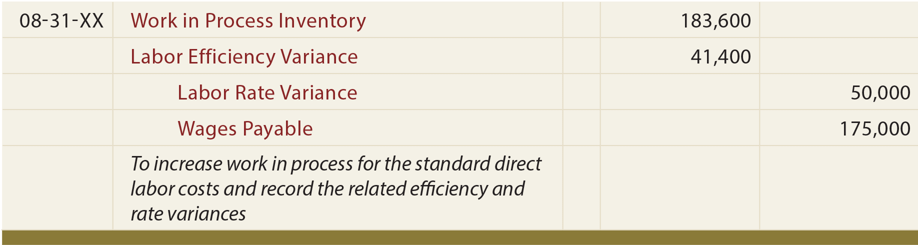
Once again, debits reflect unfavorable variances, and vice versa. Such variance amounts are generally reported as decreases (unfavorable) or increases (favorable) in income, with the standard cost going to the Work in Process Inventory account.
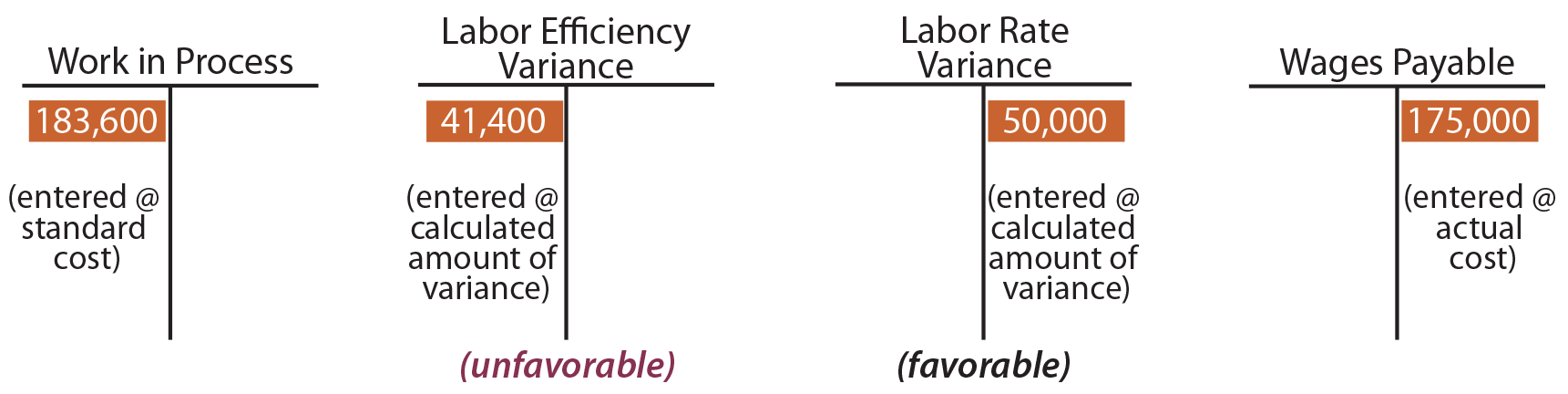
The following diagram shows the impact within the general ledger accounts:
Factory Overhead Variances
Variance analysis should also be performed to evaluate spending and utilization for factory overhead. Overhead variances are a bit more challenging to calculate and evaluate. As a result, the techniques for factory overhead evaluation vary considerably from company to company. To begin, recall that overhead has both variable and fixed components (unlike direct labor and direct material that are exclusively variable in nature). The variable components may consist of items like indirect material, indirect labor, and factory supplies. Fixed factory overhead might include rent, depreciation, insurance, maintenance, and so forth. Because variable and fixed costs behave in a completely different manner, it stands to reason that proper evaluation of variances between expected and actual overhead costs must take into account the intrinsic cost behavior. As a result, variance analysis for overhead is split between variances related to variable overhead and variances related to fixed overhead.
Variable Factory Overhead Variances
The cost behavior for variable factory overhead is not unlike direct material and direct labor, and the variance analysis is quite similar. The goal will be to account for the total “actual” variable overhead by applying: (1) the “standard” amount to work in process and (2) the “difference” to appropriate variance accounts.
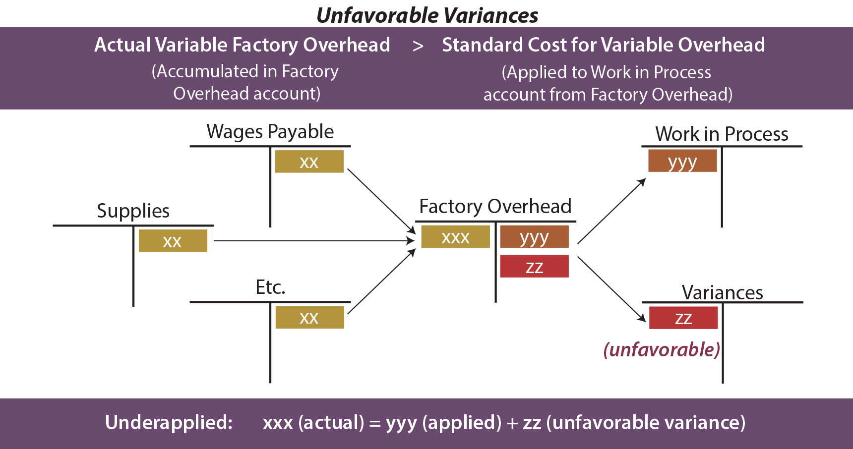
Review the following graphic and notice that more is spent on actual variable factory overhead than is applied based on standard rates. This scenario produces unfavorable variances (also known as “underapplied overhead” since not all that is spent is applied to production). As monies are spent on overhead (wages, utilization of supplies, etc.), the cost (xx) is transferred to the Factory Overhead account. As production occurs, overhead is applied/transferred to Work in Process (yyy). When more is spent than applied, the balance (zz) is transferred to variance accounts representing the unfavorable outcome.
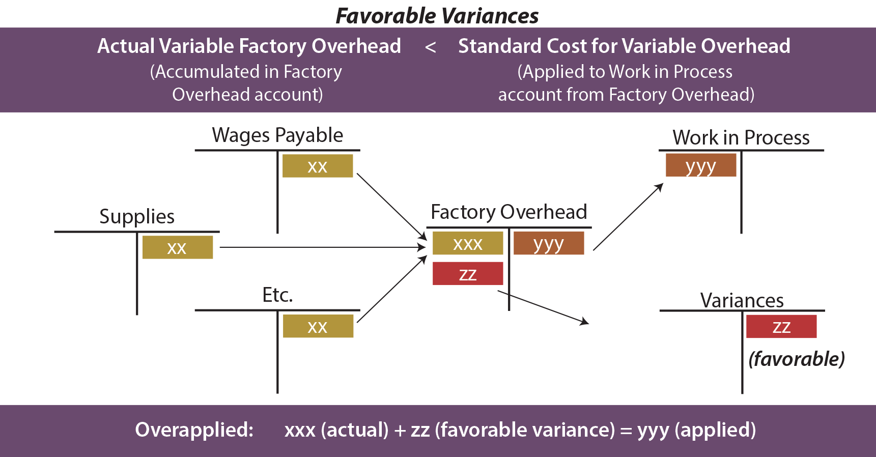
The next illustration is the opposite scenario. When less is spent than applied, the balance (zz) represents the favorable overall variances. Favorable overhead variances are also known as “overapplied overhead” since more cost is applied to production than was actually incurred.
A good manager will want to explore the nature of variances relating to variable overhead. It is not sufficient to simply conclude that more or less was spent than intended. As with direct material and direct labor, it is possible that the prices paid for underlying components deviated from expectations (a variable overhead spending variance). On the other hand, it is possible that the company’s productive efficiency drove the variances (a variable overhead efficiency variance). Thus, the Total Variable Overhead Variance can be divided into a Variable Overhead Spending Variance and a Variable Overhead Efficiency Variance.
Before looking closer at these variances, it is first necessary to recall that overhead is usually applied based on a predetermined rate, such as $X per direct labor hour. This means that the amount debited to work in process is driven by the overhead application approach. This will become clearer with the following illustration.
Case Study
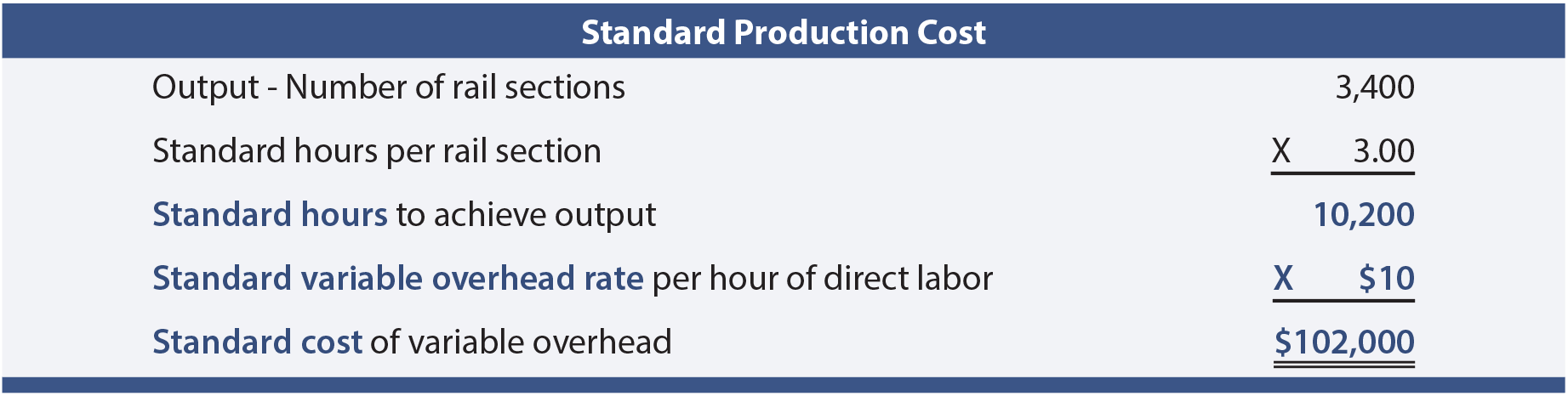
Blue Rail’s variable factory overhead for August consisted primarily of indirect materials (welding rods, grinding disks, paint, etc.), indirect labor (inspector time, shop foreman, etc.), and other items. Extensive budgeting and analysis had been performed, and it was estimated that variable factory overhead should be applied at $10 per direct labor hour. During August, $105,000 was actually spent on variable factory overhead items. The standard cost for August’s production was as follows:
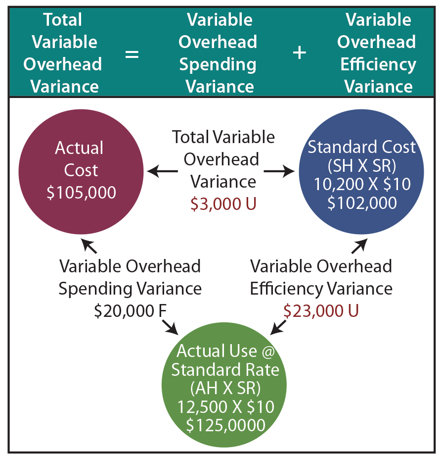 The total variable overhead variance is unfavorable $3,000 ($102,000 – $105,000). This may lead to the conclusion that performance is about on track.
But, a closer look reveals that overhead spending was quite favorable, while overhead efficiency was not so good. Remember that 12,500 hours were actually worked.
Since variable overhead is consumed at the presumed rate of $10 per hour, this means that $125,000 of variable overhead (actual hours X standard rate) was attributable to the output achieved. Comparing this figure ($125,000) to the standard cost ($102,000) reveals an unfavorable variable overhead efficiency variance of $23,000. However, this inefficiency was significantly offset by the $20,000 favorable variable overhead spending variance ($105,000 vs. $125,000).
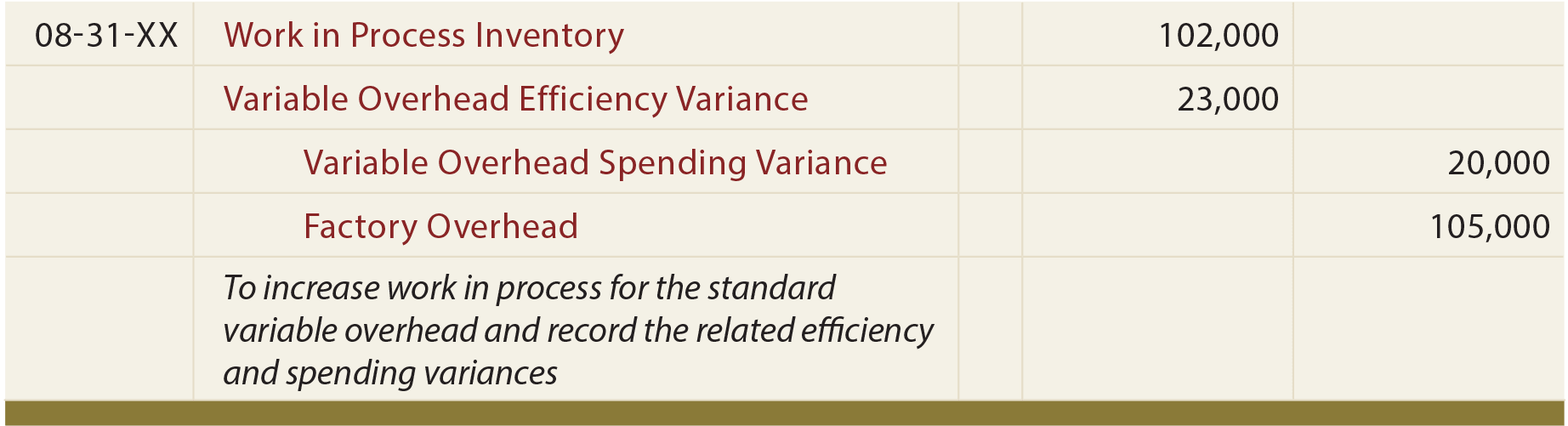
Journal Entry
This entry applies variable factory overhead to production and records the related variances:
The variable overhead efficiency variance can be confusing as it may reflect efficiencies or inefficiencies experienced with the base used to apply overhead. For Blue Rail, remember that the total number of hours was “high” because of inexperienced labor. These welders may have used more welding rods and had sloppier welds requiring more grinding. While the overall variance calculations provide signals about these issues, a manager would actually need to drill down into individual cost components to truly find areas for improvement.
Fixed Factory Overhead Variances
Actual fixed factory overhead may show little variation from budget. This results because of the intrinsic nature of a fixed cost. For instance, rent is usually subject to a lease agreement that is relatively certain. Depreciation on factory equipment can be calculated in advance. The costs of insurance policies are tied to a contract. Even though budget and actual numbers may differ little in the aggregate, the underlying fixed overhead variances are nevertheless worthy of close inspection.
Case Study
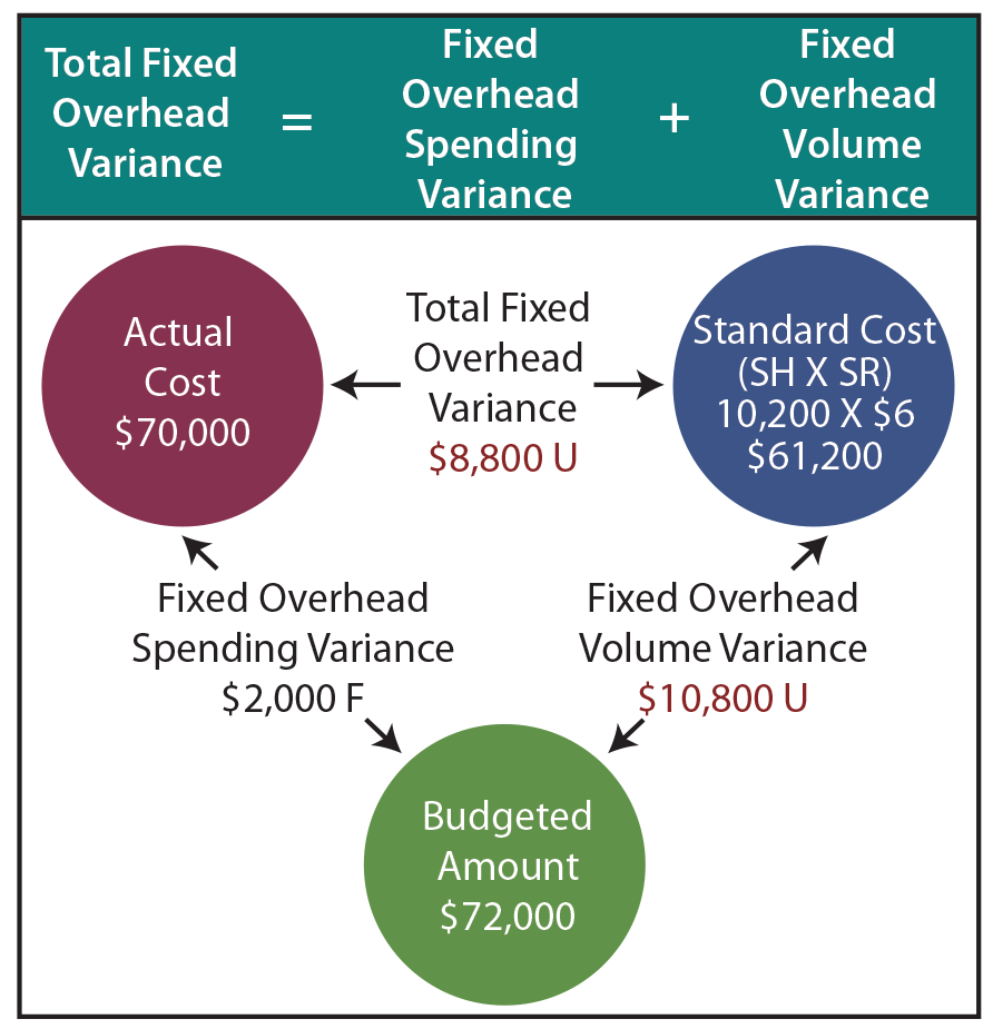 Blue Rail budgeted total fixed overhead at $72,000, but only $70,000 was spent. The objective is to allocate $70,000 between work in process and variance accounts. Work in Process should reflect the standard fixed overhead cost for the actual output. Assume that Blue Rail had planned on producing 4,000 rail systems during the month; only 3,400 systems were actually produced. This means that the planned fixed overhead was $18 per rail ($72,000 ÷ 4,000 = $18). Because 3 labor hours are needed per rail, the fixed overhead allocation rate is $6 per direct labor hour ($18 ÷ 3).
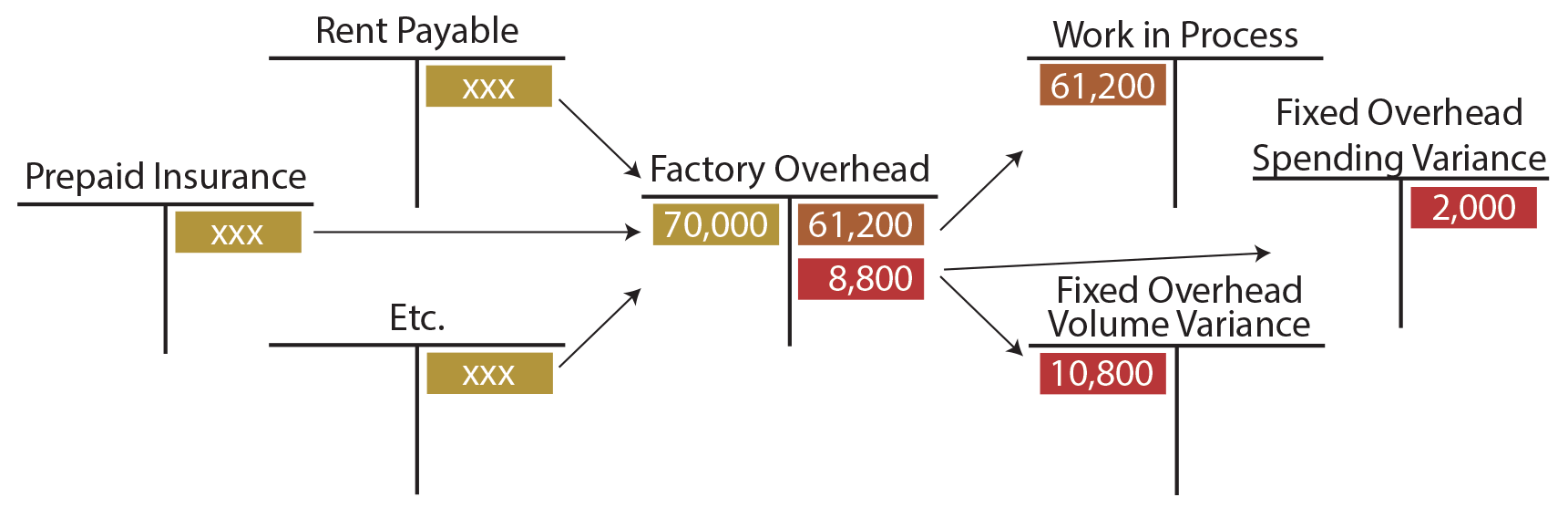
As illustrated, $61,200 should be allocated to work in process. This reflects the standard cost allocation of fixed overhead (i.e., 10,200 hours should be used to produce 3,400 units). Notice that this differs from the budgeted fixed overhead by $10,800, representing an unfavorable Fixed Overhead Volume Variance.
Since production did not rise to the anticipated level of 4,000 units, much of the fixed cost (that was in place to support 4,000 units) was “under-utilized.” For Blue Rail, the volume variance is offset by the favorable Fixed Overhead Spending Variance of $2,000; $70,000 was spent versus the budgeted $72,000. Following is an illustration showing the flow of fixed costs into the Factory Overhead account, and on to Work in Process and the related variances.
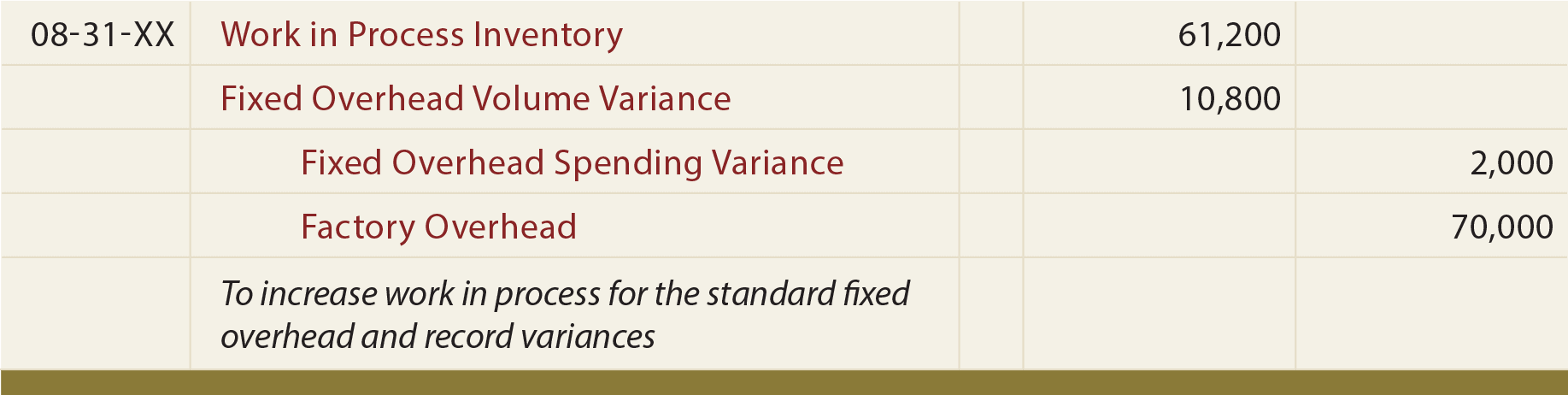
Following is the entry to apply fixed factory overhead to production and record related volume and spending variances:
Recap
The following spreadsheet summarizes the Blue Rail case study. Carefully trace amounts in the spreadsheet back to the illustrations.
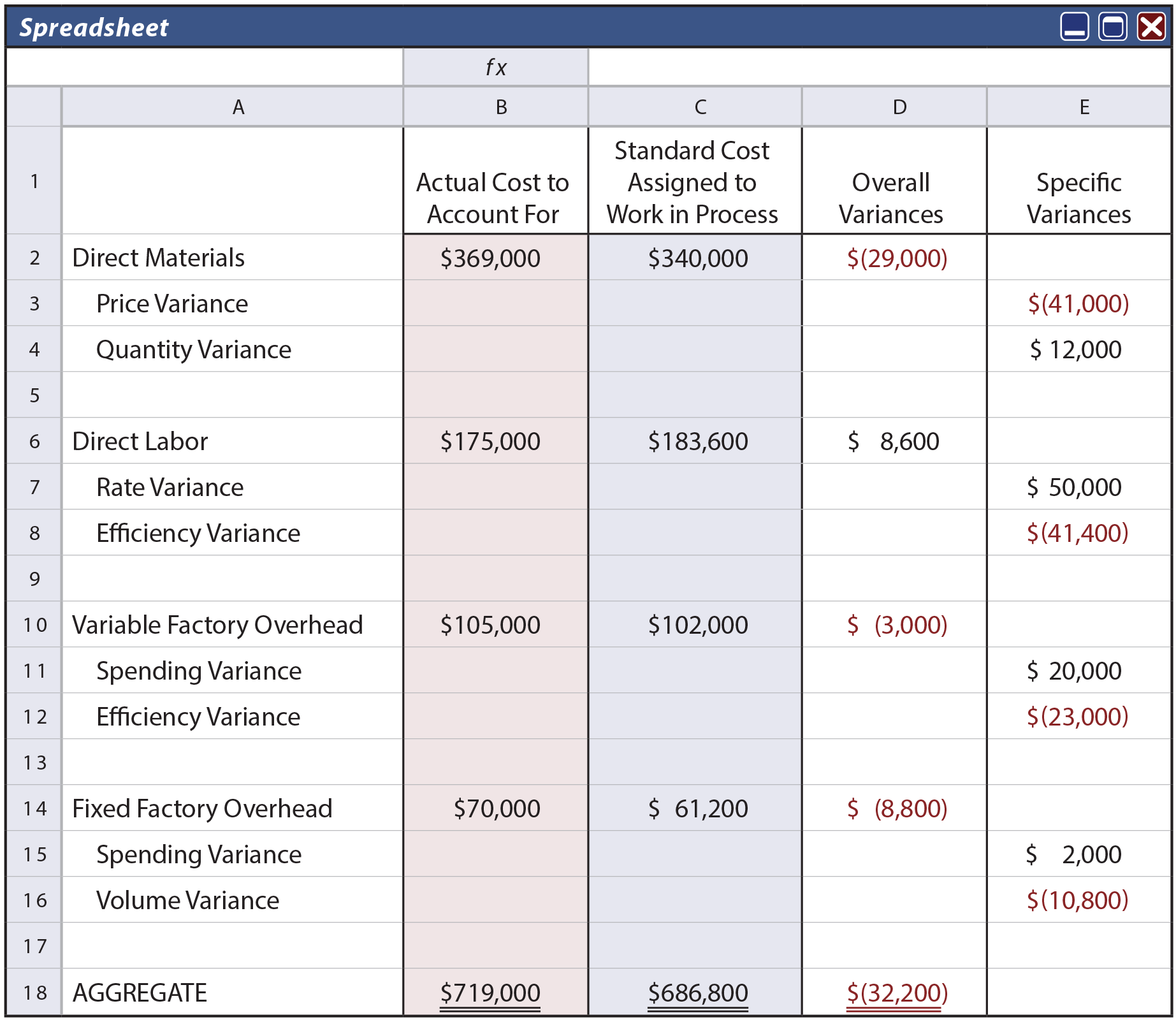
Notice that the standard cost of $686,800 corresponds to the amounts assigned to work in process inventory via the various journal entries, while the total variances of $32,200 were charged/credited to specific variance accounts. By so doing, the full $719,000 actually spent is fully accounted for in the records of Blue Rail.
Examining Variances
Not all variances need to be analyzed. One must consider the circumstances under which the variances resulted and the materiality of amounts involved. One should also understand that not all unfavorable variances are bad. For example, buying raw materials of superior quality (at higher than anticipated prices) may be offset by reduction in waste and spoilage. Likewise, favorable variances are not always good. Blue Rail’s very favorable labor rate variance resulted from using inexperienced, less expensive labor. Was this the reason for the unfavorable outcomes in efficiency and volume? Perhaps! The challenge for a good manager is to take the variance information, examine the root causes, and take necessary corrective measures to fine tune business operations.
In closing this discussion of standards and variances, be mindful that care should be taken in examining variances. If the original standards are not accurate and fair, the resulting variance signals will themselves prove quite misleading.
| Did you learn? |
|---|
| What is a variance? |
| Be able to calculate and explain material, labor, and overhead variances. |
| When should variances be investigated? |